import numpy as np
import matplotlib.pyplot as plt
from scipy.integrate import trapz # AUC
import pandas as pd
import statsmodels.api as sm
from statsmodels.formula.api import ols
import random
import copy
import statsmodels.api as sm
import statsmodels.formula.api as smfPharmacokinetic Analysis
Ref: Winnonlin Guide 8.3, Design and Analysis of Bioavailability and Bioequivalence Studies, 2×k 교차설계법에서 생물학적 동등성 추가시험의 통계적 절차, 식품의약품안전처 의약품 동등성 시험 기준
Import
PK Analysis
Generic Medicine
Bioequivalent
Drug companies must submit an abbreviated new drug application (ANDA) to FDA for approval to market a generic drug that is the same as (or bioequivalent to) the brand product3
생동성 시험은 제재학적으로 동등한 두 제제의 동등성 입증을 위해 실시하는 샐체내 실험으로, 통계학적으로 두 제제의 생체이용률의 유사성을 비교하는 시험을 의미한다.(우화형 and 박상규 2014)
Parameter
- \(AUC_t\)
- Area under the curve from the time of dosing to the time of the last measurable (positive) concentratio
- 약물 투여 시점부터 마지막으로 측정 가능한 (양수인) 농도까지의 면적인 (Area Under the Curve, AUC)는 약동학에서 사용되는 일반적인 파라미터
- 시간에 따른 약물 노출의 범위를 추정하는 데 사용
- 해당 기간 동안 혈중에서의 누적된 약물 농도를 나타냄
- \(C_{max}\) - Maximum observed concentration, occurring at time Tmax, as defined above.
- \(T_{max}\)에서의 최대 농도
- \(T_{max}\)
- Time of maximum observed concentration. For non-steady-state data, the entire curve is considered. If the maximum observed concentration is not unique, then the first maximum is used.
- 최대 혈중 농도가 관찰된 시간
- 유일한 값이 아닌 경우 첫번재 값 사용
- \(\lambda_z\)
- First-order rate constant associated with the terminal (log-linear) portion of the curve. Estimated by linear regression of time vs. log concentration
- 곡선의 말단(로그-선형) 부분과 관련된 1차 속도상수는 시간 대 로그 농도의 선형 회귀를 통해 추정
- 곡선의 로그-선형 영역에서 시간과 로그 농도 간의 선형 관계를 분석하여 얻어진 1차 속도상수
- 약동학 데이터의 로그-선형 부분에서 시간 대 로그 농도의 관계를 선형 회귀하여 추정된 1차 속도상수를 의미.
- \(ln(2)/\lambda_z\)
- Terminal half-life
- \(Tau\)
- Available in the Dosing Used results worksheet for steady-state data. The (assumed equal) dosing interval for steady-state data.
- 반복 투여하는 연구에서 반복투여하는 간격
- 예) 12시간 간격으로 하루에 두 번 투여시, tau = 12
- \(AUC_{TAU}\)
- The partial area from dosing time to dosing time plus Tau. See “Partial area calculation”
- for information on how it is computed
- tau간격 별로 혈중 농도 곡선 하 면적.
-\(\text{ Swing}\): Cmax – Cmn/Cmin
-\(\text{ Fluctuation}\)
- 100(Cmax – Cmin)/Cavg
- where Cmin and Cmax were obtained between dosing time and dosing time plus Tau
- 약물 농도의 최소값(\(C_{min}\))과 최대값(\(C_{max}\)) 사이의 변동을 약물 투여 간격 내에서 평균 농도(\(C_{avg}\))에 대한 백분율로 나타내는 약동학적 파라미터 .
약동학 파라메터 산출 프로그램 윈놀린 가이드 참고4
- page 146 정도부터 파라메터 설명 및 계산법 확인
아래는 식품의약품 안전처 규칙 내용 중 일부
- AUCt: 투약시간부터 최종 혈중농도 정량 시간 t까지의 혈중농도-시간곡선하면적
- AUC∞ : 투약시간부터 무한시간까지의 혈중농도-시간곡선하면적 (AUC∞ = AUCt + Ct/λZ
- Ct : 최종정량농도
- λZ : 말단 소실 정수
- AUCt/AUC∞ : AUCt의 AUC대한 비
- t1/2β : 소실 반감기
- AUCτ : 정상상태의 투여간격τ중의 혈중농도-시간 곡선하면적
- Cmax :최고혈중농도
- Css,max정상상태의 최고혈중농도
- Css,m: 정상상태의 최저혈중농도
동등성 기준 : Tmax를 제외한 대조약과 시험약의 비교평가항목치를 로그변환하여 통계처리 하였을 때, 로그변환한 평균치 차의 90% 신뢰구간이 log 0.8에서 log 1.25 이내이어야 한다
2 x 2 Crossover Design
현재 식품의약품 안전처에서는 두 제제의 생동성 평가 방법으로 2 x 2 교차설계법을 이용하여 두 제제의 생체이용률의 평균을 비교하는 방법 사용
| Period 1 | Period 2 | |
|---|---|---|
| Sequence 1 | Reference | Test |
| Sequence 2 | Test | Reference |
\[y_{jkl} = \mu + g_j + S_{l(j)} + p_k + \pi_{jk} + \epsilon_{jkl}\]
\[j = 1,2; k = 1,2; l=1,2, \dots, n_{1j}\]
\[S_{l(j)} \sim iid N(0,\sigma^2_s) , \epsilon_{jkl} \sim iid N(0, \sigma^2_\epsilon)\]
혈중 농도 곡선 예시
_seq = ['1'] * 18 + ['2'] * 18
random.shuffle(_seq)
seq = _seq.copy()prd = ['1', '2']# Define the two-compartment model function
def two_compartment_model(t, ka, ke, Vc, Vp, dose):
Cp = dose / (Vc + Vp) * (ka / (ka - ke)) * (np.exp(-ke * t) - np.exp(-ka * t))
return Cp# Time range
t = np.linspace(0, 24, 20) # Generate 100 time points from 0 to 24 hours# Number of subjects
n_subjects = 36# Subject-specific pharmacokinetic parameter values
ka_values = np.random.uniform(0.2, 0.8, n_subjects) # Elimination rate constant (1/hour)
ke_values = np.random.uniform(0.05, 0.15, n_subjects) # Absorption rate constant (1/hour)
Vc_values = np.random.uniform(8, 12, n_subjects) # Central volume of distribution (L)
Vp_values = np.random.uniform(3, 7, n_subjects) # Peripheral volume of distribution (L)
dose = 100 # Dose (mg)
Conc1=[]
# Calculate and plot the pharmacokinetic concentration profile for each subject
for i in range(n_subjects):
ka = ka_values[i]
ke = ke_values[i]
Vc = Vc_values[i]
Vp = Vp_values[i]
Sequence=seq[i]
period = prd[0]
Cp = two_compartment_model(t, ka, ke, Vc, Vp, dose)
Conc1.append(Cp)# Subject-specific pharmacokinetic parameter values
ka_values = np.random.uniform(0.2, 0.8, n_subjects) # Elimination rate constant (1/hour)
ke_values = np.random.uniform(0.05, 0.15, n_subjects) # Absorption rate constant (1/hour)
Vc_values = np.random.uniform(8, 12, n_subjects) # Central volume of distribution (L)
Vp_values = np.random.uniform(3, 7, n_subjects) # Peripheral volume of distribution (L)
dose = 100 # Dose (mg)
Conc2=[]
# Calculate and plot the pharmacokinetic concentration profile for each subject
for i in range(n_subjects):
ka = ka_values[i]
ke = ke_values[i]
Vc = Vc_values[i]
Vp = Vp_values[i]
Sequence=seq[i]
period = prd[1]
Cp = two_compartment_model(t, ka, ke, Vc, Vp, dose)
Conc2.append(Cp)fig, (ax1,ax2) = plt.subplots(1,2,figsize=(15,6))
fig.suptitle('Pharmacokinetic Concentration Profile (36 Subjects)')
for i in range(n_subjects):
ax1.plot(t,Conc1[i])
ax2.plot(t,Conc2[i])
ax1.set_xlabel('Time (hours), Period 1')
ax1.set_ylabel('Concentration (mg/L)')
ax2.set_xlabel('Time (hours), Period2')
ax2.set_ylabel('Concentration (mg/L)')Text(0, 0.5, 'Concentration (mg/L)')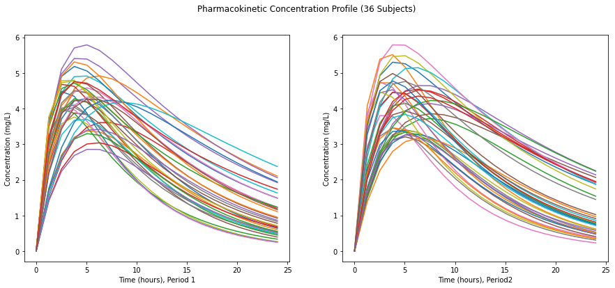
사다리꼴 공식으로 AUC 계산
auc=[]
# AUC 계산
for i in range(n_subjects):
    auc.append(trapz(Conc1, t))

auc[1]
array([56.95045738, 47.86409131, 42.21622527, 59.539426 , 86.67551908,
47.16716698, 69.1238562 , 48.31886351, 41.10456731, 77.54870044,
44.17471182, 84.86979417, 51.38750987, 56.38187092, 93.31926042,
64.86536492, 41.39841529, 49.34549501, 55.17694992, 47.80196397,
77.1173659 , 62.99088402, 67.81589046, 45.75082563, 41.08144901,
57.4092617 , 70.38694013, 60.65264211, 59.20130041, 78.037517 ,
75.13235504, 73.39727457, 45.94199314, 76.49863041, 52.37590008,
65.83072325])auc=[]
# AUC 계산
for i in range(n_subjects):
auc.append(trapz(Conc2, t))
auc[1]array([84.4561748 , 64.38750901, 64.54764973, 78.25285497, 83.33710259,
42.09336221, 39.00740636, 46.58495744, 47.68689149, 61.33957607,
49.50640257, 51.21446227, 57.54921195, 60.33096918, 75.4969536 ,
70.99863328, 49.58934078, 39.85776773, 85.49622606, 85.15095208,
44.31980906, 54.2843326 , 45.06451141, 78.41403231, 54.24686961,
57.3555638 , 91.1838877 , 73.63435573, 46.36158269, 53.44649347,
60.8944747 , 41.69662451, 77.70187433, 76.08368653, 44.59083617,
67.45281013])trapz?Signature: trapz(y, x=None, dx=1.0, axis=-1) Docstring: An alias of `trapezoid`. `trapz` is kept for backwards compatibility. For new code, prefer `trapezoid` instead. File: ~/anaconda3/envs/temp_csy/lib/python3.8/site-packages/scipy/integrate/_quadrature.py Type: function
_df = pd.DataFrame()

for i in range(n_subjects):
    temp_df1 = pd.DataFrame({
        'Subject':str(i),
        'Sequence': seq[i],
        'Period': prd[0],
        'Concentration': Conc1[i]
    })
    temp_df2 = pd.DataFrame({
        'Subject':str(i),
        'Sequence': seq[i],
        'Period': prd[1],
        'Concentration': Conc2[i]
    })
    _df = pd.concat([_df, temp_df1, temp_df2])

print(_df)
Subject Sequence Period Concentration
0 0 1 1 0.000000
1 0 1 1 2.468394
2 0 1 1 3.712638
3 0 1 1 4.216262
4 0 1 1 4.284278
.. ... ... ... ...
15 35 2 2 1.571857
16 35 2 2 1.412285
17 35 2 2 1.268903
18 35 2 2 1.140074
19 35 2 2 1.024323
[1440 rows x 4 columns]_df.loc[(_df['Sequence'] == '1') & (_df['Period'] == '1'), 'Treatment'] = 'R'
_df.loc[(_df['Sequence'] == '2') & (_df['Period'] == '2'), 'Treatment'] = 'R'
_df.loc[(_df['Sequence'] == '1') & (_df['Period'] == '2'), 'Treatment'] = 'T'
_df.loc[(_df['Sequence'] == '2') & (_df['Period'] == '1'), 'Treatment'] = 'T'_df| Subject | Sequence | Period | Concentration | Treatment | |
|---|---|---|---|---|---|
| 0 | 0 | 1 | 1 | 0.000000 | R |
| 1 | 0 | 1 | 1 | 2.468394 | R |
| 2 | 0 | 1 | 1 | 3.712638 | R |
| 3 | 0 | 1 | 1 | 4.216262 | R |
| 4 | 0 | 1 | 1 | 4.284278 | R |
| ... | ... | ... | ... | ... | ... |
| 15 | 35 | 2 | 2 | 1.571857 | R |
| 16 | 35 | 2 | 2 | 1.412285 | R |
| 17 | 35 | 2 | 2 | 1.268903 | R |
| 18 | 35 | 2 | 2 | 1.140074 | R |
| 19 | 35 | 2 | 2 | 1.024323 | R |
1440 rows × 5 columns
데이터 설명
- Subject: 대상자
- Sequence: 순서군
- Period: 시기군
- Concentration: 혈중농도
- Treatment: 치료군
# ANOVA 모델 적합
model = smf.mixedlm('Concentration ~ Treatment + Period + Sequence', data=_df, groups=_df['Subject']).fit()print(model.summary()) Mixed Linear Model Regression Results
===========================================================
Model: MixedLM Dependent Variable: Concentration
No. Observations: 1440 Method: REML
No. Groups: 36 Scale: 1.7059
Min. group size: 40 Log-Likelihood: -2460.9348
Max. group size: 40 Converged: Yes
Mean group size: 40.0
-----------------------------------------------------------
Coef. Std.Err. z P>|z| [0.025 0.975]
-----------------------------------------------------------
Intercept 2.386 0.119 19.991 0.000 2.152 2.620
Treatment[T.T] 0.055 0.069 0.804 0.421 -0.080 0.190
Period[T.2] 0.034 0.069 0.494 0.621 -0.101 0.169
Sequence[T.2] 0.005 0.154 0.033 0.974 -0.297 0.307
Group Var 0.171 0.040
===========================================================
해석
- Trearmet의 p값은 0.05보다 큼. 치료 효과는 유의하지 않다.
- Period의 p값은 0.05보다 큼, 시기효과는 유의하지 않다.
- Sequence의 p값은 0.05보다 큼, 순서효과는 유의하지 않다.
References
우화형, and 박상규. 2014. “2\(\times\) k 교차설계법에서 생물학적 동등성 추가시험의 통계적 절차.” 한국데이터정보과학회지 25 (6): 1181–93.
Footnotes
https://www.fda.gov/drugs/frequently-asked-questions-popular-topics/generic-drugs-questions-answers↩︎
식품의약품안전처 의약품 동등성 시험 기준↩︎
https://www.fda.gov/drugs/frequently-asked-questions-popular-topics/generic-drugs-questions-answers↩︎
https://onlinehelp.certara.com/phoenix/8.3/responsive_html5_!MasterPage!/WinNonlin%20User%27s%20Guide.pdf↩︎